EC102, Lab 4: Defining your own functions

[This is the fourth in a series of lecture notes for the lab component of the core ‘Macroeconomics I’ course that I teach in the M.A. Economics programme at Ambedkar University, Delhi.]

• First: Lab 1.
• Previous: Lab 3.

In the code examples that follow I assume that you have executed

import numpy as np
import matplotlib.pyplot as plt
%matplotlib inline

at the beginning of your IPython session.

Defining your own functions

So far we have been users of functions like sin from the math module or plot from the pyplot module. It is time we also become producers of functions.

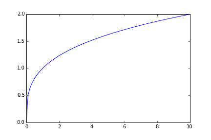
Let’s write a function that given the values of $\alpha$ and $k_{max}$ will produce a plot of the Cobb-Douglas production function $f(k)=k^\alpha$ in the range $[0,k_{max}]$.

The definition would look like:

def cobb_douglas(alpha,kmax):
    """
    Plot the Cobb-Douglas function y=k**alpha 
    for k in [0,kmax]
    """
    NPOINTS = 100
    k = np.linspace(0,kmax,NPOINTS)
    y = k**alpha
    plt.plot(k,y)

Run the block of code above in a single cell. Then run,

cobb_douglas(0.3,10)

The graph of the Cobb-Douglas function should appear.

How does this work? The keyword def on the first line tells Python that we are beginning the definition of a function. Next we give the name we want the function to have, in this case cobb_douglas. The rules for names are the same as before: upper- and lower-case letters, digits and underscores, beginning with a letter (in fact names beginning with underscores are also allowed, but they are interpreted specially by Python). After the name we give a comma-separated list of names of arguments for the function then a colon.

Following the first line ending in the colon is the actual code — or body — of the function. How does the Python interpreter know where the body of the function ends? It looks at the identation. Notice that the lines of code below the def line in the body are indented to the right by the same amount. In IPython you can get this indendtation by pressing the Tab key at the beginning of the line. When the Python interpreter is reading your code it looks at the first line following the def and sees how far it is indented to the right. Every subsequent line that is indented as far to the right as this is considered to be part of the body of the function. When the interpreter encounters a line indented by less than this amount it concludes that the body of the function has ended and the function definition is complete.

The intent behind a function definition is that the arguments to the function – in our case alpha and kmax – are unknowns whose value will be provided by the user of our function. When the user calls the function, say by running the code cobb_douglas(0.3,10), the name alpha is bound to 0.3, kmax is bound to 10 and the body of the function is run with these bindings.

Let us look more closely at the body of the cobb_douglas function. First we have

    """
    Plot the Cobb-Douglas function y=k**alpha 
    for k in [0,kmax]
    """

This is a multi-line string. Earlier we have seen that strings can be specified by enclosing text in single or double quotation marks. Such strings must end within a single line. Python allows multi-line strings to be defined by enclosing the text in three double-quotation marks. So these lines are just specifying a constant string. This seems futile as far as the goal of our computation is concerned. But this string is there to take advantage of a Python convention. If the first thing in the body of a function is a string, it is taken to be the docstring (short for documentation string) of the function. When the user requests help for the function this string is displayed to them. If you followed the example above in IPython, when you wrote the call cobb_douglas( a small window would have popped up to display this string.

Providing a docstring for a function is optional and we will not provide them for most of our examples. But it is a good practice to provide them for important functions in your code to remind yourself and others about what the function does and how it is to be used.

The next line in the definition of cobb_douglas is

    NPOINTS = 100

As usual this is an assignment statement binding the object 100 to the name NPOINTS. Yet something different and very important is going on here. The binding created by an assignment statement in the body of a function is visible only within the rest of the body of the function. We say that the scope of this binding is the rest of the body of the function.

If you try to print the value of NPOINTS outside the body of the function, Python will complain that it is undefined. This is a very important service provided by functions. As we have discussed earlier, one of the problems that a programming language must solve is the clashing of names. By making bindings in a function local to a function, we can be sure that the use of NPOINTS in this function will not clash with its use elsewhere and interfere in unexpected ways with the rest of the program to produce errors.

The bindings you create in a notebook cell have global scope, i.e. they are visible within the rest of the program, including within the body of any functions you define. So we could have put the assignment to NPOINTS outside the function (without the indent since it is no longer part of the function body) and still its use within the function body would have been fine. But you must resist as far as possible the temptation to put things in the global scope. Since global names are visible everywhere one has to study the whole program to understand their behaviour. By keeping things local we make our programs easier to understand piece-by-piece.

Why have the name NPOINTS at all? Why not just use the number 100 directly where it is required? The computer would produce the same result. But for humans reading the program the intent of the number 100 would remain mysterious. By giving it a symbolic name which conveys that it is the number of points to be plotted we make our program easier to understand for people.

The remaining code in the body of cobb_douglas creates some more local bindings and then calls the plot function from pyplot to display the graph

    k = np.linspace(0,kmax,NPOINTS)
    y = k**alpha
    plt.plot(k,y)

The pyplot library has a hidden global object that keeps track of the current figure and the plot function updates this figure. This is why our function can produce a figure that is displayed in the global scope.

This hidden global object used by pyplot goes against the approach discussed above of keeping things local as far as possible, but it is provided by pyplot for convenience when writing short programs. For larger programs, where keeping things local is more important, Matplotlib does provide altrnatives to pyplot.

Why define functions?

What are the advantages of putting the code for plotting a Cobb-Douglas graph in a function of its own? There are primarily two kinds of benefits.

First, functions allow code reuse. If we need to graph Cobb-Douglas functions many times, we need not repeat the code. We can just call the same function with different arguemnts. A common beginner error is to take some code which works and then copy and paste it whenever it is needed again. There are two problems with this. First, a reader of your code (which may be yourself a few weeks down the line) cannot easily make out what is common and what different in the two pieces of code and must therefore spend double the effort in understanding the program. Second, it is inevitable that the code will have to be changed over time to add feature and remove bugs and you must then remember to make the change in all places that the code was pasted. It is much better then to abstract away the common part of a repeated calculation in a separate function, and express the different uses in different palaces by passing in different values for arguments.

Also, it is very likely that you are not the only person in the world who needs Cobb-Douglas graphs. Once you have defined a function to produce such graphs you can share it with others. Open-source software like the Python interpreter, IPython or the NumPy and Matplotlib libraries are nothing other than such sharing taken to a high level.

The second benefit for defining function is abstraction. Having defined a function for making Cobb-Douglas graphs we can forget about its implementation and treat it as a black-box in the rest of our program. If at some other point in the program you come across the cell

cobb_douglas(0.3,10)
cobb_douglas(0.4,10)

you can just say to yourself “Ah, we are plotting two Cobb-Douglas curves” without bothering at that point about how the plotting happens. If at some other time you find you are unhappy with the Cobb-Douglas graphs produced you can go and work on the cobb_douglas function itself without worrying about how it is used elsewhere.

Abstraction also makes programs easier to write. You could start bottom up, first enriching the Python language by teaching it to draw Cobb-Douglas curves by defining functions like cobb_douglas and then writing your main program in this enriched language that is more suited to economics.

Returning values from function

The function cobb_douglas is atypical in the sense that it takes input but does not produce any direct output. Its only effect is to change the current figure displayed by pyplot. In general functions both consume inputs and produce outputs.

Consider a function that, given $\alpha$ and $k$ computes the level of per-capita output according to the Cobb-Douglas production function. We could write it as follows:

def cobb_douglas_y(alpha,k):
    """
    Return per-capita output for Cobb-Douglas
    production function y = k**alpha
    """
    y = k**alpha
    return y

The new ingredient is the return statement in the last line which consists of the keyword return followed by an expression. If when evaluating the body of the function the Python interpreter reaches a return statement it stops evaluating the body of the function and the value of the expresion after the return keyword becomes the value of the function. So after defining the function above if we evaluate

cobb_douglas_y(0.3,4)

we would get the result 1.515716566510398.

The result of a function call can not only be printed, it can be used like any other value to build up more complicated expressions. So, the following would be meaningful expressions

output = cobb_douglas_y(0.3,4)
(1-s)*cobb_douglas_y(0.3.4)

Returning multiple objects

The cobb_douglas_y functions returns just a single object – a number. Sometimes you may want to return multiple objects froma a function. Formally in Python a function can return only a single object. But that’s not a problem. To return multiple objects we just pack them together in a single collection object such as a list, tuple or array. For example the function

def square_n_cube(x):
    return x**2,x**3

returns a tuple the first element of which is the square of this argument and the second element the cube. If you evaluate square_n_cube(3) the result will be the tuple (9,27).

There is an extension of the assignment statement which is very useful when dealing with functions returning multiple values as tuples. If you have a list of names separated by commas on the left-hand side of an assignment and on the right-hand side an expression yielding a tuple with the same number of elements as the number of names on the left-hand side then each name on the left gets bound to the corresponding element of the tuple on the right. In short

s,c = square_n_cube(3)

binds s to 9 and c to 27.