[This is the fifth in a series of lecture notes for the lab component of the core ‘Macroeconomics I’ course that I teach in the M.A. Economics programme at Ambedkar University, Delhi.]

• First: Lab 1.
• Previous: Lab 4.

In this session we will look at how to use the SciPy package to explore systems of differential equations.

At the beginning of your session run the following imports:

import numpy as np
import matplotlib.pyplot as plt
import scipy.integrate as spint
%matplotlib inline

Systems of differential equations

A system of differential equations is of the form

$$\frac{dx}{dt} = f(x,t)$$

where $x$ is a vector in $\Re^n$ and $f$ is a function from $\Re^n \times \Re$ to $\Re^n$. If $f$ does not actually depend on $t$ the differential equation system is said to be autonomous, otherwise nonautonomous.

A solution to this differential equation system is a function $\phi(t)$ from some time interval $[t_0,t_1]$ to $\Re^n$ such that

$$\phi'(t) = f(\phi(t),t)$$

Usually there are many solutions to a differential equation system, and we need to impose additional conditions to pick a unique solution. For example, we may impose an initial condition

$$\phi(0)=x_0$$

where $x_0$ is a given point in $\Re^n$.

For most differential equation systems it is not possible to find an explicit formula for the solution. However, for many systems it is possible to use computers to find approximate numerical solutions to systems of differential equations.

Numerical solutions

A single differential equation

The function odeint in the module scipy.integrate provides a user-friendly interface computing for numerical solutions of differential equations. The function takes three essential parameters:

odeint expects that func will be a function whose first two arguments will be the current state $x$ (which is in general n-dimensional) and time $t$ respectively and which will return the right-hand side of the differential equation system (another n-dimensional vector). When using odeint we do not call f ourselves. Rather we provide it to odeint which calls it as required to compute the numerical solution.

Let’s try out the function on the one-dimensional autonomous system

$$dy/dx = -5y$$

with the initial condition $y_0 = 1$.

def f(y,t):
    return -5*y
t = np.linspace(0,1,5)
y0 = 1
y = spint.odeint(f,y0,t)

Note that we have to define f as a function of both y and t even though we do not use t in the function as our differential equation system is autonomous. This is because odeint expects f to have a particular form.

The array t gives the time points for which we would like to know approximate values of the solution. For our experiment we choose five equally-spaces points between 0 and 1.

If you check after runnning the code above, y.ndim is 2 and y.shape is (6,1). In general the return value of odeint is two dimensional, with one row for each time point at which we asked for a solution and one column for each variable in our system.

For future work let’s convert y into a 1-d vector

y = y[:,0]

Something new here. y[:,0] is a subscript operation, but instead of specifying a row by using an integer, we provide the special symbol : which in NumPy means all rows. And we provide 0 as the column number to pick only the first column. So we get a 1-d vector which just has the first column from each row.

In this example we chose a differential equation whose solution we can compute in terms of a formula. For the initial value $y_0=1$ the solution is $e^{-5t}$. If you want you can compute np.exp(-5*t) and compare the answer with the value y computed above. The numbers will not be exactly the same, since odeint does not know the exact formula and must compute an approximation, but they should be close.

A multi-dimensional system

Solving a differential equation system in more than one dimension follows the same pattern, except that for a n-dimensional system the function passed to odeint must be written to accept a n-element array as the state variable and must return the right-hand side of the differential equation system as another n-element array.

Suppose we want to study the system

$$dx/dt = y;\qquad dy/dt = -x-0.2y$$

with the initial condition $x_0 = 0, y_0=1$.

The Python code will be

def f(s,t):
    xdot = s[1]
    ydot = -s[0]-0.2*s[1]
    return np.array([xdot,ydot])
t = np.linspace(0,10,50)
s0 = np.array([0,1])
s = spint.odeint(f,s0,t)

We call the first argument to f as s to remind ourselves that it is the 2-element array containing the state of the system, with its first element s[0] being $x$ and its second element s[1] being $y$. We return the 2-element vector whose elements are $dx/dt$ and $dy/dt$.

$s$ is now a 2-d array with shape (50,2). To visualize the trajectory of this system we plot the consecutive value of $x$, given by s[:,0] against the consecutive values of $y$ given by s[:,1].

plt.plot(s[:,0],s[:,1])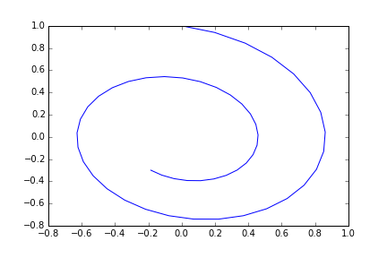

Differential equations with parameters

Suppose we want to replace the second equation in the system above with

$$dy/dt = -ax - by$$

where $a$ and $b$ are parameters for which we would like to try out different values. The f function would then be rewritten as

def f(s,t,a,b):
    xdot = s[1]
    ydot = -a*s[0]-b*s[1]
    return np.array([xdot,ydot])

By default odeint calls the function we provide only with the state and the time, which would not work in this case. For such situations, odeint as an additional argument args which takes a tuple which is interpreted as additional arguments to be provided in the call to f. So we could get the same plot as before by executing, with the new definition of f:

t = np.linspace(0,10,50)
s0 = np.array([0,1])
s = spint.odeint(f,s0,t,args=(1,0.2))

Suppose we would like to compare the trajectories for $b=0.2$ and $b=0$. We call odeint twice with the two paramter values and then plot both the trjectories in the same figure.

s_first = spint.odeint(f,s0,t,args=(1,0.2))
s_second = spint.odeint(f,s0,t,args=(1,0))
plt.plot(s_first[:,0],s_first[:,1],label="0.2")
plt.plot(s_second[:,0],s_second[:,1],label="0.0")
plt.legend()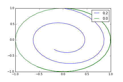

Visualizing vector fields

Vector field plots are another way to visualize a autonomous 2-dimensional differential equation system. Let’s consider again the equation system

$$dx/dt = y; \qquad dy/dt=-x-0.2y$$

At every $(x,y)$ point the right-hand side of these equation give us the direction of motion of the trajectory of the system passing through that point. So we if have a good idea of how the direction of motion varies in different parts of the plane we will also have a good idea of the shape of the trajectories. Vector field plots help in this by representing the direction of motion at selected points by arrows. pyplot contains a convenient function quiver for drawing such plots, but it requires a bit of setup. We give the code and the plot before getting into the description.

x = np.linspace(-1,1,10)
y = np.linspace(-1,1,10)
xx,yy = np.meshgrid(x,y)
xdot = yy
ydot = -xx-0.2*yy
plt.quiver(xx,yy,xdot,ydot)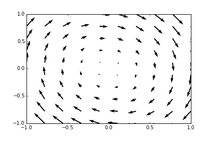

Now the description. The two lines

x = np.linspace(-1,1,10)
y = np.linspace(-1,1,10)

sets up two equally spaced 1-d vectors of x- and y-coordinates with 10 elements each. But what we need is a 10×10 2-d grid of points at which to draw our arrows. The NumPy function meshgrid does precisely this, taking two 1-d grids, using them to form a 2-d grid and then returning a tuple of two elements the first of which contains the x coordinate at all points of the grid and the second contains the y coordinates at all point in the grid.

xx,yy = np.meshgrid(x,y)

Here we have an example of using the extended form of the assignment statement to take apart the tuple returned by mesgrid and assigning its two element to two different names.

Then we compute $dx/dt$ and $dy/dt$ at each point in the grid

xdot = yy
ydot = -xx-0.2*yy

Element-by-element arithmetic works for the 2-d arrays xx and yy just like it worked in our earlier 1-d examples. Finally we call quiver

plt.quiver(xx,yy,xdot,ydot)

quiver has four essential arguments: x coordinates at grid points, y coordinates at grid points, the x component of the arrows and the y component of the arrows. Here the two components of the arrows come from the right-hand side of a differential equation system, but quiver does not care where they come from. quiver automatically scales the arrows so that their direction remains unchanged but their sizes span a reasonable range.

Exercises

Exercise 1

Consider the differential equation system

$$dx/dt = x+y;\qquad dy/dt = x-y$$

On a single figure plot

1. The vector field for $-1 \le x \le 1$, $-1 \le y \le 1$
2. The trajectory with initial value $(-0,4.1)$.
3. The trajectory with initial value $(0.5,-1)$.

Exercise 2

For $u(c)=c^{1-\theta}/{1-\theta}$ and $f(k) = k^\alpha$, the Ramsey model’s trajectories are given by the equations

$$dc/dt = \frac{c}{\theta}[\alpha k^{\alpha-1}-\rho]$$ $$dk/dt = f(k)-c-nk$$

Take $\alpha=0.3$, $\theta=1.75$, $\rho=0.05$ and $n=0.01$.

1. Use Python to compute the steady state values $c^*$ and $k^*$.
2. Suppose we want to visualize the phase portraits of the model. What are the reasonable ranges for $c$ and $k$ for our plot.
3. On one diagram plot the vector field correspoinding to the differential equation and a few sample trajectories.
4. Add to the above diagram dashed vertical and horizontal lines corresponding to $k^*$ and $c^*$ respectively.
5. It is hard to plot the stable arm directly as we don’t know what initial value to choose and even the slightest error or numerical approximation will lead to the path exploding. However there is a useful trick available. We know that the stable arm converges to the steady state. So if we start somewhere near the steady state and run time in reverse we should get approximately the stable arm. Try this trick to plot the stable arm.