Solving the competitive storage model using collocation

The original Python notebook is on Github. Download it if you would like to follow along.

This IPython notebook solves the competitive storage model for the price of storable commodities using collocation as the numerical method. We reproduce an example from section 9.9.2 of Miranda and Fackler’s Applied Computational Economics and Finance using Python and independently of the authors’ CompEcon MATLAB toolbox.

The problem

The competitive storage model is a simple model for the price of a storable commodity. It has an uneven empirical record but it provides a good illustration of the computational problems which arise in modern macroecnomics.

We consider a commodity, say wheat, which can be stored subject to the condition that a fraction $\lambda$ of the total stock at the end of a period disappears before the beginning of the next period and a cost per unit cost $c$ has to be paid for storage. In each period there is an addition to stocks due to a stochastic harvest $z$ and a reduction in stock from an outside demand given by a demand function $P(q)$ .

Storage decisions are taken by competitive speculators who must form expectations about future prices. These future prices depend on both the stochastic harvest in the next period as well as the total stock carried forward by all speculators taken together. We assume that speculators have rational expectations.The speculators are assumed to be risk neutral and discount their future profits by a discount factor $\delta$ .

Let $s_t$ be the stock at the beginning of period $t$ and $x_t$ be the stock at the end of period $t$ and $p_t$ be the price that prevails in period $t$ . Then the equilibrium conditions are, first that outside consumers should demand the quantity $(s_t-x_t)$ that is not stored,

$p_t = P(s_t-x_t)$

that the stocks in consecutive periods be linked according to the storage technology, $s_{t+1} = (1-\lambda)x_t+z_{t+1}$

and most importantly the speculators maximize profits. $p_t \ge \delta(1-\lambda)[E_t p_{t+1}]-c,\quad \text{with equality if $x_t>0$}$

The last equation has the complementary slackness form it has becuase speculators may be at a corner solution where they do not carry forward any stocks at all. If this is the case then current prices can rise above the expected future return from carrying stocks. On the other hand current prices can never be lower than expected future revenues in equilibrium since such a condition would produce an infinite demand for wheat by speculators in the current period.

The solution algorithm

It is known that the above system of equations has a solution of the form $p_t = \phi(s_t)$ . However there is generally no analytical solution and the function $\phi(\cdot)$ must be computed numerically.

Suppose we expect that prices next period are governed by the function $f(s_{t+1})$ . Then the price function this period, say $g(s_{t})$ , will be a function of this expectation through our equilibrium conditions above. We express this relationship in the form

$g = Tf$

where $T$ is an abstract operator representing the working of the equilibrium conditions. It is precisely the property of a stationary rational equations solution that it is a fixed-point of this operator

$\phi = T\phi$

i.e., the expected law of prices is such as to produce behaviour which confirms the expect law of prices.

In order to find an approximate solution to this fixed-point equation we restrict our search to the finite dimensional space of Chebyshev polynomials of a given degree. The true solution may not lie in this space and thus no function in this space may satisfy the fixed-point equation at all points. In order to nonetheless get a good approximation to the true solution the collocation method we use in this notebook requires that the function come close to satising the fixed-point equation at a given finite set of points. In this notebook we take these points to be Chebyshev nodes. The task of finding the Chebyshev polynomial which satisfies this condition is carried out through successive approximation: starting from an initial guess $f_0$ we calculate $y_n = (Tf_0)(x_n)$ at our chosen Chebyshev nodes $x_n$ . Then $f_1$ is then taken to be a Chebyshev polynomial that passes through the points $(x_n,y_n)$ . This is continued until we reach a fixed point.

There are two more technical difficulties. The operator $T$ involves computing a conditional expectation in order to find expected profits. For arbitrary functions this cannot be done exactly and we have to make a numerical approximation. In this notebook we use Gauss-Hermite quadrature to replace the continuous distribution of the shocks $z_t$ by a discrete approximation.

Finally, we need to work with a bounded state space for our calculations. If $\lambda>0$ and $\bar z$ the maximum possible realization of the shock then the beginning-of-period stock can never exceed $\bar z/\lambda$ . This however does not work when $\lambda=0$ . Also using this bound is harmful even when $\lambda>0$ since this forces us to consider very large values of stock which are not reached in equilibrium, thereby wasting computational resources. We therefore follow the literature in arbitrarily assuming that there is an upper abound $x_{max}$ on end-of-period stocks. The value of this parameter is adjusted to be large enought that it is never reached in equilibrium.

See Judd, Numerical Methods in Economics, Chapter 11 and 17 for more details as well as alternative algorithms. Section 17.4 discusses the competitive storage model.

Imports

import sys
import math as m
import numpy as np
from numpy import linalg
import scipy.optimize as spopt
from numpy.polynomial.chebyshev import Chebyshev
from numpy.polynomial.hermite import hermgauss
from scipy.stats import rv_discrete
import scipy.io as spio
import matplotlib.pyplot as plt
from collections import namedtuple
%matplotlib inline

Collocation

Collocation in general

def collocation_solve(T,fhat,nodes,fit,
                      log=True,tol=1e-6,maxiter=500):
    """
    Try to solve the operator equation Tf = f.
    We use successive approximations to find a function fhat in some function
      space such that Tfhat = fhat at all points in `nodes`.
      
    Inputs:
    
    T(fhat,s): return (Tfhat)(s)
    fhat: initial guess for fhat
    nodes: collocation nodes
    fit: a function when called as fit(x,y) with x and y 
         as arrays, returns an element phi of the chosen
         function space such that phi(x[i]) = y[i]
    log: if True prints progress messages
    tol: tolerance parameter for stopping criteria
    maxiter: maximum number of successive approximation 
             iterations to try
             
    Returns:
    
    Either `fhat` if success or `None` if iteration count exceeded.
    """
    
    for i in range(maxiter):
        lhs = np.empty_like(nodes)
        rhs = np.empty_like(nodes)
        for j,s in enumerate(nodes):
            lhs[j] = T(fhat,s)
            rhs[j] = fhat(s)
        err = linalg.norm(lhs-rhs,np.inf)
        if log and i%10==0:
            print("Iteration {}: Error = {:.2g}".format(i+1,err),
                  file=sys.stderr)
            plt.plot(nodes,lhs,"b-",label="Tf")
            plt.plot(nodes,rhs,"r-",label="f")
            plt.legend()
            plt.show()
        fhat = fit(nodes,lhs)
        if err<tol:
            return fhat
    if log:
        print("collocation_solve: iteration count exceeded",
              file=sys.stderr)
    return None

Collocation using Chebyshev polynomials and nodes

def chebyshev_solve(T,guesser,degree,domain,
                    log=True,tol=1e-6,maxiter=500):
    """
    Try to solve the operator equation Tf = f using
    Chebychev collocation.
    
      
    Inputs:
    
    T(fhat,s): return (Tfhat)(s)
    guesser: a function, `guesser(x)` gives  a guess 
             for the function at point `x`.
    degree: the degree of the Chebyshev series to use
    domain: a list `[lower,upper]` of the domain over 
            which the function is to be approximated
    log: if True prints progress messages
    tol: tolerance to be used in stopping criteria
    maxiter: maximum number of iterations for successive 
             approximation.
    
    Returns:
    Either `fhat` if success or `None` if iteration count 
    exceeded.
    """
    
    nodes = Chebyshev.basis(degree+1,domain).roots()
    
    def fitter(x,y):
        return Chebyshev.fit(x,y,degree,domain)
        
    f0 = fitter(nodes,
                np.array([guesser(n) for n in nodes]))
                
    return collocation_solve(T,f0,nodes,fitter,log,tol,maxiter)

The competitive storage model

The problem data structure

# A competitive storage problem
StorageProb = namedtuple("StorageProb",
                        ["cost"   # Marginal cost per-unit stored
                        ,"shrink" # Fraction of goods lost per period ($\lambda$)
                        ,"yvol"   # Log of harvest is distributed N(0,yvol)
                        ,"xmax"   # Maximum end-of-period stock
                        ,"disc"   # Time discount rate ($\delta$)
                        ,"P"      # External demand function P(q)
                        ])

Solution

# Solving the problem
class StorageSolution(object):
    """
    A solution to the competitve storage model.
    
    Constructor:
    
    StorageSolution(prob,hgdeg=5,cdeg=50,
                    tol=1e-6,maxiter=500,log=True)
        
        hgdeg: degree of Gauss-Hermite 
               discretization of shocks
        cdeg: dgree of Chebychev polynomial to use
        tol: tolerance for stopping criteria
        maxiter: maximum no of iterations 
        log: if True print progress report
    
        The model is solved in the process of constructing 
        the object, so constructor calls are expensive.
        
        If the model cannot be solved in the give number of 
        iterations throws a ValueError. Computational 
        problems can cause an AssertionError to be thrown.
    
    Instance variables:
    
    Saved from constructor: prob, hgdeg, cdeg, tol
    
    Others:
    
        smax       Maximum beginning-of-period stock
        smin       Minimum beginning-of-period stock
        zs         An array of discretized harvest shock values
        ws         An array of probability weights 
                   corresponding to `ws`
        
        phi        The computed price as a function of 
                   begining-of-period shocks
        
        storage_revenue(phi,x)
                    Discounted expected revenue net of storage 
                    costs per unit stored when the pricing 
                    function is `phi` and end-of-period stocks
                    in the current period is `x`.
        
        opti_storage(phi,s)
                    The optimal amount to store when the pricing 
                    function is `phi` and beginning-of-period 
                    stocks is `s`. Rational expectations is
                    built in: the expected stocks tomorrow is 
                    consistent with storage decision taken.

        T(phi)      We want T(phi,s) = phi(s) for all s.
    """
    
    def __init__(self,p,ghdeg=5,cdeg=50,
                 tol=1e-6,maxiter=500,log=True):
        
        # Store input parameters
        self.prob = p
        self.ghdeg = ghdeg
        self.cdeg = cdeg
        self.tol = tol
        
        # Compute Gauss-Hermition integration nodes
        ys,self.ws = hermgauss(ghdeg)
        self.ws = self.ws/m.sqrt(m.pi)
        self.zs = np.exp(ys*p.yvol)
        zmin,zmax = np.min(self.zs), np.max(self.zs)
        
        # Bounds for beginning-of-period stocks
        # Note xmax is maximum end-of-period shocks
        self.smin = zmin
        self.smax = zmax + (1 - p.shrink)*p.xmax
        
        # Storage revenue computation
        def storage_revenue(phi,x):
            Etom = sum(
                        phi(z + (1 - p.shrink)*x)*w 
                        for (z,w) in zip(self.zs,self.ws)
                        )
            return p.disc*(1 - p.shrink)*Etom - p.cost
                
        self.storage_revenue = storage_revenue
        
        # Optimal storage decision
        def opti_storage(phi,s):
            P = p.P
            xmax = p.xmax
            
            if s>xmax and storage_revenue(phi,xmax) > P(s-xmax):
                return xmax
            elif storage_revenue(phi,0) < P(s-0):
                return 0
            else:
                max_feas = min(xmax,s)
                x_star,r = \
                    spopt.brentq(lambda x:\
                                     storage_revenue(phi,x)-P(s-x),
                                 0,max_feas,
                                 full_output=True,
                                 xtol=1e-5)
                assert r.converged
                return x_star
            
        self.opti_storage = opti_storage
            
        # Initial guess for pricing function
        def init(s):
            return p.P(s)
        
        # We want T(phi) = phi
        def T(phi,s):
            x_star = opti_storage(phi,s)
            ans = p.P(s-x_star)
            assert ans>=0
            return ans
        self.T = T
        
        self.phi = chebyshev_solve(T,init,cdeg,
                              [self.smin,self.smax],
                              log,tol,maxiter)
        if self.phi is None:
            raise ValueError("Failed to converge")

Visualization and simulation

def illustrate(soln):
    """
    Plot solution variables and diagnostics
    ``soln` is an instance of `StorageSolution`
    """
    f,((ax1,ax2),(ax3,ax4)) = plt.subplots(2,2,sharex=True)
    f.set_size_inches(10,10)
    
    ss = np.linspace(soln.smin,soln.smax,100)
    
    store = [soln.opti_storage(soln.phi,s) for s in ss]
    ax1.plot(ss,store)
    ax1.set_title("Equilibrium storage")
    ax1.set_xlabel("Supply")
    ax1.set_ylabel("Storage")
    
    P = [soln.prob.P(s) for s in ss]
    phi = [soln.phi(s) for s in ss]
    ax2.plot(ss,P,"r-",label="without storage")
    ax2.plot(ss,phi,"b-",label="with storage")
    ax2.legend()
    ax2.set_title("Equilibrium price")
    ax2.set_xlabel("Supply")
    ax2.set_ylabel("Price")
    
    def optimal_profit(s):
        x = soln.opti_storage(soln.phi,s)
        return soln.storage_revenue(soln.phi,x)-soln.prob.P(s-x)
    profits = [optimal_profit(s) for s in ss]
    ax3.plot(ss,profits)
    ax3.set_title("Arbitrage profit")
    ax3.set_ylabel("Profit")
    ax3.set_xlabel("Supply")
    
    resid = [soln.T(soln.phi,s)-soln.phi(s) for s in ss]
    ax4.plot(ss,resid)
    ax4.set_title("Approximation residual")
    ax4.set_ylabel("Tf-f")
    ax4.set_xlabel("Supply")

def simulate(soln,niter,burnin=1000,s0=None):
    """
    Run a simulation.
    
    soln: An instance of `Storage Solution`
    niter: The number of iteration for which to return results
    burnin: The number of initial iterations to discard
    s0: Initial beginning-of-period stock. 
        None selects the middle point of the domain.
        
    Returns: arrays x and P of end-of-period stocks and prices
    
    """
    
    xs = np.empty(niter)
    Ps = np.empty(niter)
    
    if s0 is None:
        s = (soln.smin+soln.smax)/2
    elif s0 > soln.smax:
        s = soln.smax
    elif s0 < soln.smin:
        s = soln.smin
    else:
        s = s0
        
    dist=rv_discrete(values=(range(len(soln.ws)),soln.ws))
    phi = soln.phi
    opti_storage = soln.opti_storage
    shrink = soln.prob.shrink
    zs = soln.zs
    P = soln.prob.P
    
    for i in range(niter+burnin):
        x = opti_storage(phi,s)
        z = zs[dist.rvs(size=1)]
        if i>burnin:
            xs[i-burnin] = x
            Ps[i-burnin] = P(s-x)
        s = (1-shrink)*x+z
    return xs,Ps

Example from Miranda & Fackler

def isoelastic_demand(gamma):
    return lambda q: q**(-gamma)

# Example from section 9.9.2 of Miranda & Fackler
mirfac_p = StorageProb(cost = 0.1,
                       shrink = 0,
                       P = isoelastic_demand(2.0),
                       yvol = 0.2,
                       xmax = 0.9,
                       disc = 0.9)
mirfac_s = StorageSolution(mirfac_p,tol=1e-10)

Iteration 1: Error = 0.14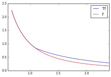

Iteration 11: Error = 1.6e-08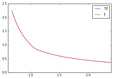

illustrate(mirfac_s)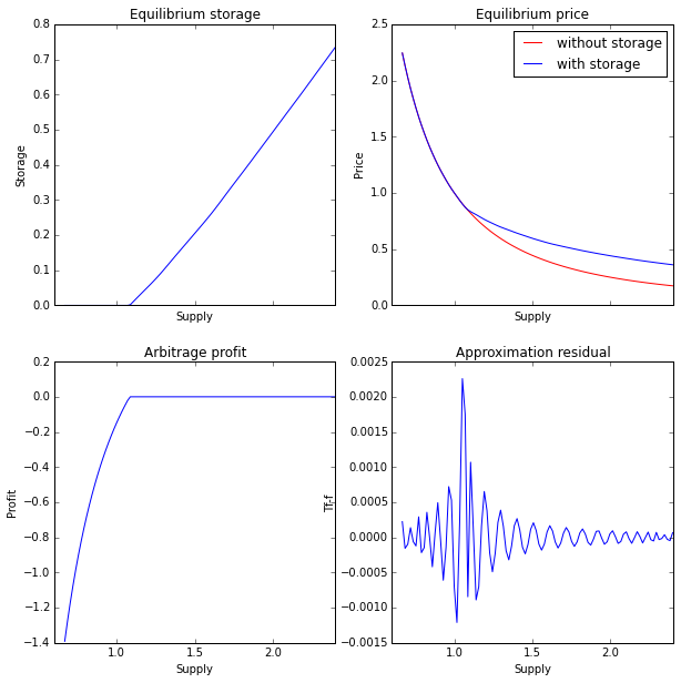

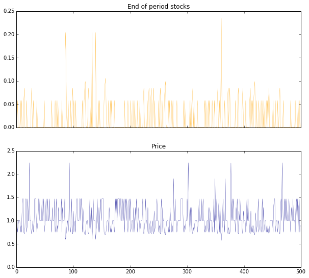
sim_N = 500
sim_xs,sim_Ps = simulate(mirfac_s,sim_N)
sim_so = (1-float(np.count_nonzero(sim_xs))
            /sim_N))
print("Proportion of stockouts = {}".format(sim_so)
f,(ax1,ax2) = plt.subplots(2,1,sharex=True)
f.set_size_inches(10,9)
ax1.plot(sim_xs,linewidth=0.3,color="orange")
ax1.set_title("End of period stocks")
ax2.plot(sim_Ps,linewidth=0.3,color="darkblue")
ax2.set_title("Price")

Proportion of stockouts = 0.71





<matplotlib.text.Text at 0x7f475ed685c0>